Wednesday 3 February 2016

Let's Write A Raytracer Part 2 : (CPU) kd Trees

Let's back away from GPU ray tracing for a second. Noting the performance of the (oh so basic) ray tracer from the last article, I grew curious about just how much better, or worse, CPUs are at tracing rays than GPUs. In addition, because CPUs let you write the software in a full, unrestricted language like C++ it's a much more enjoyable experience. Let's get started then.

I've created a GitHub repo for this project, which you can find here.

CPU Raytracer Architecture
I'll describe the ray tracer architecture as it is at this point in time, but check the git log itself for any further updates.

Let's start with the main component, the abstract Raytracer class. This class defines the interface that the application can use to render scenes. It also contains pointers to the camera, frame buffer and scene objects. Why is it abstract? Because there's several ways that we can generate rays to create our final image. For instance, you can multi sample for each pixel, you can process the framebuffer in a tiled manner, you can process rays using one or more CPU cores etc. It currently has one concrete implementation class, BasicRaytracer which generates and processes pixels using a single thread, in  scanline order, and with one sample per pixel (hey it's called "basic" for a reason!).

The FrameBuffer class contains the memory that will be rendered into, and methods for saving its contents to a .tga file afterwards. Nothing special here.

Now for the tricky part, and this is best explained with the help of a class diagram:


Any object that accepts a ray and does some work with implements the ITraceable interface.
As you can see, IScene is traceable, but also defines the interface for a collection of ITraceable objects. This makes sense if you consider that a ray can then just be passed into a scene, which contains other objects, themselves which are traceable.

The BoundedTraceable class simply defines a traceable object with an axis-aligned bounding box added for culling and intersection purposes, what space (object/world) these bounding boxes represent varies depending on context. Unlike the GPU raytracer, we don't simply transform all the triangles that make up the scene into world space prior to intersection testing. Here we have the core geometry objects themselves defined in object space in the standard way and we transform the rays from world space into object space prior to any triangle intersection tests. This is what the GeometryInstance class does, it contains the world space orientaiton, position and scale (represented in a Basis class) of a piece of geometry, and transforms rays into object space prior to passing them off to the contained *Geometry class. There are two of these currently, the BasicGeometry class which simply stores a list of triangles to intersect with, and the KdTreeGeometry class which stores the triangles in a kd tree acceleration structure. More on that later.

Let's evaluate the performance of running the most basic combination in the new system, using the BasicGeometry structure all rays have to test against the entire set of the triangles that comprise the Blender Monkey mesh. For a 1280x720 scene shown here:


rendering time takes around 18.5 seconds.As this is on an AMD Bulldozer CPU we can pretty much divide those results by 6 (or 8) for a parallel implementation. In the best case this is still around 2.3 seconds for a single frame. Hardly real time I'm sure we all agree.

Kd Tree Acceleration
The next thing to do is an investigation into acceleration structures for the triangle meshes that comprise our scene geometry. There are a number of them out there but kd trees are the generally accepted best solution.

Kd trees are simple enough in concept. They are binary space partitioning (BSP) trees that restrict the choice of splitting planes to be aligned with one of the three axes, and where only the leaf nodes of the tree contain any geometry. You have a k-dimensional region of space, and you subdivide it by splitting it along one of its cardinal axes at each level of a binary tree. If you're not familiar with the concept it takes a little bit of visualization. Imagine you have a rectangular region of space, and you want to carve it up so you only consider smaller regions of space at a time. You start by picking an axis to subdivide along, say the x-axis. You carve space into two regions along that axis and store them in the child nodes of the root node of the tree. Then for each of those child nodes, pick an axis, say the y-axis, and subdivide again. See below:


You repeat this until you reach some termination criterion. This can be that less than a certain number of triangles are contained in the node, or that the maximum tree depth is reached. More on the construction algorithms and their resulting performance later.

Kd Tree Traversal
How do kd trees accelerate the time it takes to determine the closest ray intersection?
For each kd tree node you have the following pieces of information at hand:

  • The bounding box encapsulating the node and all of its children;
  • The splitting plane;
  • The incoming ray.

The basic idea is to use the above to compute three t values for the incoming ray that correspond to points of interest in relation to the kd tree node (where the points are defined by ray_position + ray_direction * t). The t values are where the ray enters the bounding volume of the kd tree node, where it intersects the splitting plane of the kd tree node (if it does indeed intersect the splitting plane), and finally where it exits the bounding volume of the kd tree node. Using these t values we can determine the optimal ordering for traversing the nodes, and can possibly even remove entire nodes from further consideration. Consider the below configurations:

tExit > tPlane > tEntry:
Traverse the current side first, before traversing the opposite side.
Ray does not intersect splitting plane so no need to consider opposite side.
tSplit > tExit:
 No need to consider opposite side.


tSplit < tEntry:
No need to consider the current side.
Note how the "current side" is defined as the side of the splitting plane that the ray position is in.
When you reach a leaf node, you run through its list of triangles and intersect against them. When the current side child node reports an intersection, you don't need to descend into the opposite side node as by definition the current side child is closer than the opposide side child. The only gotcha that you need to watch out for is when a child node reports an intersection, but the returned intersection point is on the opposite side of the splitting plane. This can happen when a triangle extends into both child nodes. It's possible for a triangle in the opposite node to actually be obscuring the current point, so you need to descend into that node as well to be sure.

In the codebase, the intersection routine is found as an implementation of the IKdTreeTraversal interface, called KdTreeStackTraversal. It's a recursive function, which is probably sub-optimal but good enough for now.

Kd Tree Construction
The choice of splitting plane axis and position, as well as how deep the resulting kd tree is for a particular dataset, has a substantial impact on the final performance of the algorithm. I've implemented two construction algorithms that you can toggle between in the codebase. The first I called naive spatial median, and the second is based off of the surface area heuristic.

The naive spatial median algorithm simply constructs a kd tree to a specified depth by dividing the node in half at every iteration and then for the final leaf nodes determining which triangles overlap them. It's simple to implement and results in a vast improvement over the flat list of triangles approach. However, evenly splitting the dataset along an axis isn't the optimal solution as it doesn't deal with uneven distributions of geometry. And providing the tree depth as an input to the algorithm might result in trees that are too shallow or too deep (and this will vary from dataset to dataset). The kd tree algorithm takes time to process at each level of the traversal stage, and this cost can result in a slower search than if the tree were shallower.

The surface area heuristic algorithm attempts to create an optimal tree by factoring in at each iteration of the kd tree construction, whether or not it would be more beneficial to subdivide the node, or to create a leaf node. Let me see if I can sum this up in a paragraph. The core idea is that, at any level of the kd tree, there is a choice between subdividing further, or simply creating a leaf node for the current region. If you choose to create a leaf node, the cost of processing a ray if it were to reach the node is simply the estimated time it takes to intersect a ray with a triangle, multiplied by the number of triangles in the leaf. The second option is to subdivide, in which case the cost of processing a ray can be estimated as the cost of processing the traversal step, plus the probability that the ray will intersect each of the child nodes, multiplied by the cost of making the child nodes leaves (we don't consider the cost of subdividing them further at this level, as that would complicate the algorithm too much). To sum up:

leaf_cost = triangle_intersection_cost * num_triangles;

subdivide_cost = traversal_cost + probabilityA * (num_triangles_a * triangle_intersection_cost) + probabilityB * (num_triangles_b * triangle_intersection_cost);

You don't have to provide "accurate" (whatever that means in the context of differing CPUs anyway) costs for the traversal_cost and triangle_intersection_cost numbers, rather it's the relative cost that is important. Is your triangle intersection code faster than your traversal step? Then set it to an appropriate fraction of the cost of the traversal step.

The probabilities are where the surface area part of the algorithm comes into play. Geometric probability theory tells us the following:
Assume you have a random ray that passes through a convex volume A.
Assume that you have another convex volume B that is contained in convex volume A.
Then the probability that the random ray will also pass through convex volume B is the surface area of B divided by the surface area of A.

For an axis aligned bounding box, its surface area can be computed as 2 * ((width * height) + (width * length) + (height * length)).

So when you choose your splitting plane, you get two resulting sub-volumes of the current node, and can compute their surface areas, number of overlapping triangles, and their corresponding probabilities. That's great, but how do we choose the correct splitting plane? There's an infinity of possible positions for it along the intervals of the bounding volume of the node you're currently evaluating. But again, smart people who have come before us have already determined that the only candidate splitting positions that actually have an effect on the final cost are the minimum and maximum triangle vertex positions on our axis of choice. (Tip: Compute the bounding volume for each of the triangles of the mesh at the beginning and use their min/max elements.)

I'm describing the SAH algorithm in context of accelerating a triangle mesh here, but it's capable of being extended to the entire scene as well if you use kd trees as your scene subdivision. I haven't done it yet, but check the repo at a later stage.

I might have confused you more than helped you with this explanation. Sorry about that, but it's hard to try and convey complicated algorithms in a couple of sentences sometimes. If you're really interested in writing something yourself though, you're going to be reading the proper academic papers along with this and then it will hopefully make much more sense. Speaking of which, most of my knowledge for building this thing came from a mighty tome called "Physically Based Rendering From Theory To Implementation". Do yourself a favour and go and purchase this book (link), as it contains the most useful and easy to digest knowledge on the subject of raytracing, kd tree construction included.

Performance
Performance improvements with kd trees are substantial. With the naive spatial median constructed kd tree rendering time fell to ~790 milliseconds for a single core (~23.5x faster). This was for a hand tuned kd tree depth, as fast as I could make it. Switching to the SAH and that number falls further to ~615 milliseconds (~30x faster). Were you to parallelise that across 6 or 8 cores you'd have a result that is competitive with the GPU raytracer results on a GTX760 from the last article. How interesting...

Thursday 5 November 2015

Short-circuit evaluation is not always your best friend.

Whilst doing some code reviews the other day I came across a piece of code that (structurally) looked like this:

if (value1 & value2 & value3)
{
    // Do something
}
else
{
    // Do something else.
}

I initially thought this was a harmless typo. If you were trying determine if 3 boolean values happened to all be true this would evaluate the same as if you had used the logical && operator ((0x01 & 0x01 & 0x01) == (true && true && true)).

Fair enough, I thought, but out of interest I wondered how different this would appear at the assembly level, so I opened up Visual Studio's disassembler. The results were very interesting. I created  a simple program that does comparisons on 3 different boolean values from 3 different arrays in a loop and increments one of two counters depending on whether or not all three elements are true:

bool g_Array1[NUM_ELEMENTS];
bool g_Array2[NUM_ELEMENTS];
bool g_Array3[NUM_ELEMENTS];

// Initialize to random values.

int numPassed = 0;
int numFailed = 0;

for (int i = 0; i < NUM_ELEMENTS; i++)
{
    if (g_Array1[i] AND g_Array2[i] AND g_Array3[i])
        numPassed++;
    else
        numFailed++;
}

Let's focus on the inner loop's generated code:

Bitwise AND

 for (int i = 0; i < NUM_ELEMENTS; i++)
008D10AE  xor         ecx,ecx  
 {
  if (g_Array1[i] & g_Array2[i] & g_Array3[i])
008D10B0  mov         al,byte ptr [ecx+9C75B0h]  
008D10B6  and         al,byte ptr [ecx+0ABB7F0h]  
008D10BC  test        byte ptr [ecx+8D3370h],al  
008D10C2  je          main+57h (08D10C7h)  
   numPassed++;
008D10C4  inc         esi  
  else
008D10C5  jmp         main+58h (08D10C8h)  
   numFailed++;
008D10C7  inc         edi  
 for (int i = 0; i < NUM_ELEMENTS; i++)
008D10C8  inc         ecx  
008D10C9  cmp         ecx,0F4240h  
008D10CF  jl          main+40h (08D10B0h)  
 }

This is as one would expect. Load the first boolean value into a register, perform a bitwise AND with the second, and finally test (set the contents of the status register to the result of the AND of) the third boolean value. This is followed by a jump to increment the correct counter.

Logical AND

 for (int i = 0; i < NUM_ELEMENTS; i++)
00F210AE  xor         eax,eax  
 {
  if (g_Array1[i] && g_Array2[i] && g_Array3[i])
00F210B0  cmp         byte ptr [eax+0F23370h],0  
00F210B7  je          main+5Eh (0F210CEh)  
00F210B9  cmp         byte ptr [eax+110B7F0h],0  
00F210C0  je          main+5Eh (0F210CEh)  
00F210C2  cmp         byte ptr [eax+10175B0h],0  
00F210C9  je          main+5Eh (0F210CEh)  
   numPassed++;
00F210CB  inc         esi  
  else
00F210CC  jmp         main+5Fh (0F210CFh)  
   numFailed++;
00F210CE  inc         edi  
 for (int i = 0; i < NUM_ELEMENTS; i++)
00F210CF  inc         eax  
00F210D0  cmp         eax,0F4240h  
00F210D5  jl          main+40h (0F210B0h)  
 }

In this context, we see something strange. The logical AND forces a comparison/potential branch for every argument in the comparison. Now conventional wisdom says to make sure your code is as branch free as possible (Modern high frequency, deeply pipelined CPUs like being able to prefetch and execute instructions well in advance and branching introduces an element of uncertainty into the process), but there is a reason for the code to be this way.

C like languages use an idiom called "short-circuiting" in the evaluation of their logical operator statements. What it entails is that evaluation of the arguments of a logical operation will only happen to the point where the result of the comparison can be determined. For example if you have an AND comparison to test if 100 arguments are all true, and the first argument evaluates to false, there will be no point in wasting time evaluating the other arguments. Likewise for the logical OR operator, which will jump to its "true" branch as soon as one of its arguments evaluates to true. This is a good thing if determining your arguments is a potentially expensive operation. After all, if you use your imagination a little, your code could potentially need to do this:

if (FetchFromDatabase() && LinkedListTraverse() && CreateNewFile())

However, for operations involving simple arguments, short-circuiting isn't optimal.

The only question left is just how much performance could you possibly gain by this kind of micro optimization? I set the size of the arrays in my test program to a million elements, populated with random boolean values. The loop we discussed is performed on them, and timings taken.
The program is so simple, I won't bother including code, just the final results.

For the logical AND evaluation, the time taken in the loop is ~7.10 milliseconds.

For the bitwise AND evaluation, the time taken in the loop drops to ~2.4 milliseconds.

That's almost 3x as fast in this case (Proportional to the number of branches in the loop?).
This code was executed on a desktop grade CPU, so it's not unreasonable to imagine that results on simpler architectures would be higher.

Wednesday 11 March 2015

Let's Write a Ray Tracer Part 1: First Rays.

With OpenGL 4.3, we finally have access to compute shaders and all of the glorious GPGPU functionality that modern hardware allows. Now, I have done some work with OpenCL before but having compute functionality that is properly integrated into the OpenGL pipeline was what finally convinced me that I should take a stab at writing a real time ray tracer that runs on the GPU.
Let's get started!

What I'm going to show you here is an introduction to the general idea of the technique, the code framework and some fundamental math required in order for us to get a basic ray tracer up and running with compute shaders. As the series progresses we'll cover more advanced topics.

What Do You Need To Know?
I am assuming that the reader is familiar with intermediate linear algebra, OpenGL and its associated shading language GLSL, some 3D mathematics (camera transforms, coordinate spaces, projection transforms etc), and basic lighting calculations. I'd love to make posts that cover all of these required topics, but I'm afraid that approaches writing a book in scope, which would require me to quit my day job and charge everyone for this! If you're not yet comfortable with those topics, go run through some of those tutorials first, perhaps get a good book or two (some are listed in my previous posts if I remember correctly), and then come on back :)

What Is Ray Tracing?
In order to properly explain what ray tracing is, we need to do a quick summary of the relevant aspects of computer graphics.

Our modern computer imagery is what you would call raster based. This means that our images consist of a generally rectangular arrangement of discrete picture elements. So all image generation algorithms we care about create images by populating each of these raster elements with a certain color.

Up until recently, rendering raster computer graphics in real time has been done mostly (pretty much exclusively) by a technique called rasterization. Rasterization is an example of an object order algorithm, whereby to draw a scene, you iterate over all of the objects in the scene and render them accordingly. The "objects" we are referring to are geometric primitives (usually triangles) which are projected onto the image plane, after which the spans of pixels that those objects cover are filled in. GPUs were initially created to perform this rasterization, and its associated operations, in hardware.
The reason why rasterization has been the preferred approach to real time rendering thus far is because the algorithm simplifies rendering in several ways, and exploits the principle of coherence to increase efficiency beyond any other approach. An explanation is beyond the scope of this post, but please check the further reading section. Primitives and their associated spans of fragments (potential pixels) are rendered in isolation, without needing to be aware of other scene elements. The results are then converged at appropriate places in the pipeline to ensure that the final image is correct.

Example of a modern rasterization pattern.

This pattern is to maximize memory coherency, which helps the algorithm's
efficiency on modern GPU memory architectures.

Image: IEEE Xplore
However, because rasterization relies on several simplifying assumptions, it gets far more complicated to do complex effects. For instance, implementing correct transparency and reflections are hard to do with the traditional rasterization approaches. Phenomena like shadows, are done using various techniques that can be quite fragile and require a good deal of tweaking to look acceptable. Other phenomena like ambient occlusion are sometimes done using screen space information only. Furthermore, as geometry density increases and triangles become less than a pixel in size, modern rasterization hardware efficiency decreases.

Ray tracing takes a fundamentally different approach to generating images. Ray tracing is an image order algorithm, which means that instead of iterating over objects in the scene, you iterate over the image elements (pixels) themselves. The way ray tracing works is that for every pixel in the scene, you shoot a ray from the camera point through its position on the projection plane and into the scene. There the ray can intersect with scene geometry. From the intersection point on the geometry you are then free to perform shading calculations and/or reflect the ray off into the scene further. Ray tracing is a more physically accurate method of generating images as the rays themselves are aware of all of the elements of the scene and the algorithm can take this into account when performing its calculations. For instance, when a ray intersects a curved transparent object, the ray itself can refract through the object and into the scene again, resulting in properly simulated light refraction. Another example would be how shadows are calculated, instead of using volume or raster based approaches, you simply cast a ray from the point on the object towards a prospective light source, and if the ray intersects some geometry, that point is in shadow.

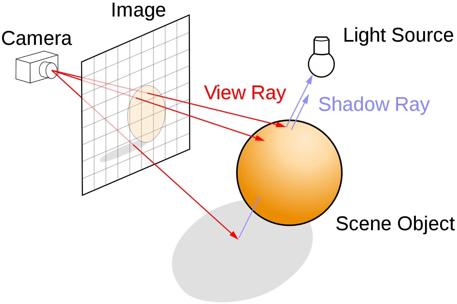
Ray tracing algorithm illustrated.

Image: Wikipedia
Ray tracing is less efficient than rasterization for generating images, especially as more complicated effects require that several rays being cast per pixel. It can require many more calculations per pixel, and because rays can be wildly divergent in terms of what they hit, it doesn't exploit coherence well. However, it is far simpler to model complex phenomena, and the algorithm scales well to parallel hardware architectures. In fact, ray tracing belongs to that rare breed of algorithm that scales almost perfectly linearly with the amount of processing elements that it is given. It is partially because of these reasons that ray tracing (or related techniques) is preferred over rasterization for offline, photo-realistic rendering.
Of course, no technique exists alone in a vacuum, and there have been several hybrid approaches that try to combine the best of both rasterization and ray tracing.  Newer PowerVR demos are utilizing what appears to be hardware accelerated ray tracing for transparencies, reflections and shadow calculations. A few other approaches worth mentioning, as dangling threads to follow up for the interested, are Voxel Cone Tracing for global illumination and Sparse Voxel Octrees for infinite geometric detail.

I should add here that another advantage that ray tracing could be said to have is that it is not restricted to rasterizable geometry (pretty much only triangles). However, for much of my purposes this is mostly useless. Most realistic scenes don't consist solely of "pure math objects" like spheres and tori!

Further Reading
http://ocw.mit.edu/courses/electrical-engineering-and-computer-science/6-837-computer-graphics-fall-2012/lecture-notes/MIT6_837F12_Lec21.pdf

http://ieeexplore.ieee.org/ieee_pilot/articles/96jproc05/96jproc05-blythe/article.html#fig_6

http://en.wikipedia.org/wiki/Cone_tracing

http://blog.imgtec.com/powervr/understanding-powervr-series5xt-powervr-tbdr-and-architecture-efficiency-part-4

 https://www.youtube.com/watch?v=LyH4yBm6Z9g

http://www.eetindia.co.in/ART_8800696309_1800012_NT_e092890c.HTM

GPU Hardware Evolution and the Emergence of Compute
We now have an idea of what ray tracing is and how it differs from rasterization. But how will it be possible to accelerate this algorithm on hardware that was architected to accelerate the rasterization
algorithm? Let's cover some history quickly.

The first truly integrated GPU that contained all components of the graphics pipeline in hardware can be traced back to as recently as late 1999 with the release of the GeForce 256. Previous video cards lacked hardware acceleration of some stages like Transform and Lighting (T&L) and therefore could not be considered true GPUs. Further development of the GPU would see the addition of multiple parallel processing units that exploited the parallelism of computer graphics operations. For example, having more than one T&L engine that could process several vertices at once. Or more than one pixel engine that could process several fragments at once. These early GPUs were fixed function as the operations that they performed on data were predetermined in hardware with very limited customizability.

The next evolution for GPUs was the addition of programmable stages in the graphics pipeline. Hardware T&L was replaced with vertex shaders, and pixel engines were replaced with fragment shaders. These vertex and fragment shaders were programs, written in a shading language that would execute on the data being fed to the graphics pipeline, allowing for custom operations to be performed.

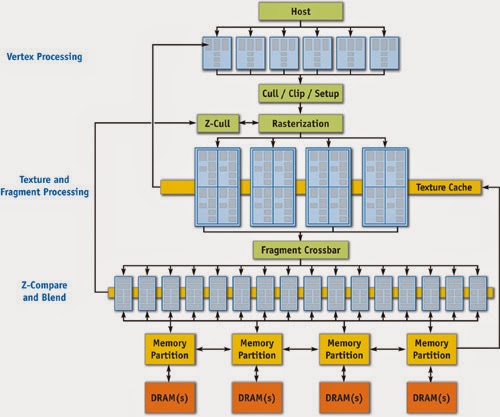
GeForce 6 Series Architecture

Here you can see the parallel and programmable processing units used for vertex and fragment processing.

Image: Nvidia
In addition to this programmability, hardware vendors soon realized that they could cater to the needs of both vertex shading and fragment shading with one hardware core, and unified shaders were born.  This trend towards increasingly general computation and unified hardware compute units has led to the modern style of graphics processor, which can be considered a massive array of general compute resources (a sea of processors) that have specific graphics related hardware attached (texture sampling units etc). Because of all this general purpose compute power available, APIs like OpenCL have been created that can take advantage of the GPU not for graphics but for general compute tasks. Although it's important to note that OpenCL isn't built for GPUs specifically. It's built to enable parallel heterogeneous computing on a wide variety of different hardware, including CPUs and DSPs.

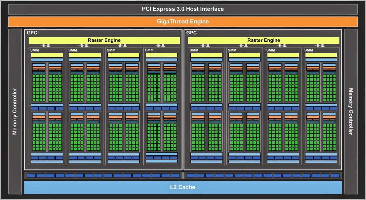
Nvidia Maxwell Architecture Diagram

Note the shift away from specialized processing units to more general units.

Image: Nvidia
The latest OpenGL version (4.3 at the time of writing) provides a feature called Compute Shaders, which are written in the OpenGL shading language but are capable of performing general computations that need not be related to rendering at all, and are not bound to a particular stage of the graphics pipeline. The big positive is how tightly integrated this functionality is with traditional OpenGL functionality. There is no need to mess around with OpenCL-OpenGL interop and contexts etc. We can use this compute functionality to do pretty much anything so long as we can express the problem in the right way. Fortunately a ray tracer is easy to express with compute shaders. We'll cover how to accomplish this in code later.

Further Reading

http://www.nvidia.com/content/GTC-2010/pdfs/2275_GTC2010.pdf

http://www.techspot.com/article/650-history-of-the-gpu/

Code Architecture Quick Description
Firstly, you should download the code and assets here

I won't cover all of the code (you can just download it and see it for yourself) but I will go through some of the various pieces to help you understand everything. The usual disclaimer about "use the code for whatever you want but don't blame me if something goes wrong" applies. The code was written with Visual Studio 2013 so you'll need that version or newer to open up the solution file.

Let's cover main.cpp first:
This is obviously the entry point for the application. I used SDL 2 and glew to handle all of the OpenGL and window related set up that we need.

Let's cover the interesting code:

    
    CameraLib::Camera camera;
    camera.ResetCameraOrientation();
    camera.SetPosition(0.0f, 0.0f, 50.0f);
    camera.SetCameraYFov(60.0f);


This sets up the camera that we'll view the scene from. My camera system is based on the OpenGL camera system exactly, as in, it is right handed and the negative z-axis in camera space contains the visible parts of the scene. The Camera class contains all of the math required to set up the camera in the virtual scene and provides convenience methods for transforming between camera and world space (as well as frustum generation methods for frustum culling etc, but that's not really useful to us for now).

    
    Raytracer::CameraControl cameraControl(camera);


This is the simple update mechanism for the camera in the scene (the camera is used by the CameraControl object and also by the ray tracer itself). The main loop accepts SDL key commands and sets state on this object, which then updates the camera every frame. Simple simple!

   
    Raytracer::Raytracer raytracer;
    raytracer.ResizeViewport(1280, 720);
    raytracer.SetCamera(&camera);


This sets up the ray tracer itself, as you can see, I've hard coded the resolution to be 1280 by 720 for now. Also, we give the ray tracer a const pointer to the camera so that it can determine where the scene is being viewed from.
   
    MathLib::quaternion identityQuaternion;
    MathLib::quaternion_setToIdentity(identityQuaternion);

    Assets::MeshManager::GetInstance().SetMeshDatabase("test.mdb");

    // Prepare scene geometry.
    raytracer.ClearSceneData();
    Raytracer::StaticMeshInstance meshInstance("monkey",
                                               MathLib::vector4(0.0f, 0.0f, 0.0f, 1.0f),
                                               identityQuaternion,
                                               5.0f);
    raytracer.AppendStaticMeshInstanceToSceneData(meshInstance);
    raytracer.CreateNewSceneDataSSBO(); 


Ok now here is where things get tricky. I use my good old trusty math library (see my first two posts ever) pretty much in all of my 3D projects. Here you can see, I create an identity orientation quaternion.

Then afterwards you can see that I initialize something called a mesh database. What this is, is that ray tracing spheres is pretty damn boring, and it's also not very useful. Most of the cool geometry created by artists or modellers these days is mesh based. So I hijacked the asset code from my main project to load up some triangle meshes for me to use.

Then after that, you can see I clear any scene data the ray tracer might have, instantiate an instance of a mesh called "monkey" at a basic orientation and position in the world and load the ray tracer with it before rebuilding something called a "Scene Data SSBO". What's happening here?

Firstly, the way I architected the ray tracer for now (and bear in mind that this is NOT the right way to go about it, but is quick and easy for me and you first time around :) ) is that all the ray tracer sees is a giant list of triangles in world space that it then intersects its rays with. So what is happening is that the ray tracer is taking the mesh instance and transforming all of it's triangles into world space and storing them in a big list somewhere, before transferring them to this SSBO thing. What is that?
That's a Shader Storage Buffer Object, and it's a new feature in OpenGL 4.3 that lets you create arrays of data and, in a shader, read those arrays of data as C-struct like arrays. It's how we can give data to the ray tracer without it being a set of hard coded spheres like every first ray tracer demo...


After that's done the main loop begins and we are away.

Raytracer class:
The ray tracer itself is ridiculously simple at heart, let's look at the main loop for instance:

 
    void Raytracer::Render()
    {
        RaytraceScene();

        TransferSceneToFrameBuffer();
    }


That's all it does guys (aside from the mundane setting up operations etc).
But to be more specific, what is actually going on is RaytraceScene() executes a compute shader which has access to that flat list of world space triangles and some camera parameters (which I'll explain later). That compute shader writes to a texture object using some new GLSL image store operations. And after that's done, we simply draw that texture over the screen as a quad.
Couldn't be simpler.

Having said that there is some OpenGL 4.3 specific stuff happening and it's beyond the scope of this post to be an OpenGL tutorial as well... I will however link to some in the further reading section. Generally though, if there's something you don't understand, just Google the function call and investigate around, it's all straight forward.

Shaders:
In the code there's also ShaderManager/ShaderProgram/Shader classes. These are just typical convenience classes used to load up shader files, compile them, link them, and provide methods to set uniform variables of various data types. The code is fairly straight forward and is lifted from my other projects (albeit expanded to support compute shaders as well).

Further Reading

http://web.engr.oregonstate.edu/~mjb/cs475/Handouts/compute.shader.1pp.pdf

 https://www.opengl.org/wiki/Compute_Shader

http://www.geeks3d.com/20140704/tutorial-introduction-to-opengl-4-3-shader-storage-buffers-objects-ssbo-demo/ 

Generating Rays
The first piece of magic that we're going to need here is the ability to generate for every pixel on the screen, an appropriate viewing ray in world space.

Specifically, we need a mechanism that:
Takes a window coordinate, in our case a value in the range [0, 1280) for the x-axis, and [0, 720) for the y-axis, and generates a ray world space for us. We are going to accomplish this with the use of two matrix transforms that can happen in the compute shader for every pixel.

The first transform that we're going to need is one that, given a 4D vector <xcoord, ycoord, 0, 1>, gives us the location in camera space of the associated point on the near projection plane.
This is better explained with the aid of a diagram, and in two dimensions.

 
Say we have the window coordinate < don't care, 0 > (which is any pixel on the top scan line of your display, remember pixels increase their position as they move to the bottom right of the screen). What we want for that y coordinate is to get the top value on our near clipping plane.
We're going to accomplish this in two steps.. firstly we're going to map the range in window coordinates from [0, width) and [0, height) to [-1, 1] each.
Following this with a scale to the top (and for the x-axis values, right) values (my camera system uses a symmetric frustum so the left most value is simply -right).

Firstly, we stick our window coordinate in a 4D vector <xcoord, ycood, 0, 1>.
Then we'll have the normalization matrix which get's us to the range [-1, 1]:

            
            MathLib::matrix4x4 screenCoordToNearPlaneNormalize
            (
                2.0f / (m_ViewportWidth - 1.0f), 0.0f, 0.0f, -1.0f,
                0.0f, -2.0f / (m_ViewportHeight - 1.0f), 0.0f, +1.0f,
                0.0f, 0.0f, 0.0f, -nearPlaneDistance, 
                0.0f, 0.0f, 0.0f, 1.0f
            );


After that we need a transform to map that normalized set of values to the correct near plane dimensions:

            
            float aspectRatio = (float)m_ViewportWidth / (float)m_ViewportHeight;

            float halfYFov = m_Camera->GetYFov() * 0.5f;

            float nearPlaneDistance = m_Camera->GetNearClipPlaneDistance();
            float top = nearPlaneDistance * tan(MATHLIB_DEG_TO_RAD(halfYFov));
            float right = top * aspectRatio;

            MathLib::matrix4x4 screenCoordToNearPlaneScale
            (
                right, 0.0f, 0.0f, 0.0f,
                0.0f, top, 0.0f, 0.0f,
                0.0f, 0.0f, 1.0f, 0.0f,
                0.0f, 0.0f, 0.0f, 1.0f
            );


These two matrices combine to give us our first required matrix:

            
            MathLib::matrix4x4 screenCoordTransform;
            MathLib::matrix4x4_mul(screenCoordToNearPlaneScale, screenCoordToNearPlaneNormalize, screenCoordTransform);
            

Excellent, now that we can get the position on the near plane for every pixel on the screen, all that is required is to be able to transform this into world space. But remember, we need to build a ray here, so what we need is to consider the position on the near plane as a direction. So we need to simply transform this by the camera's orientation matrix:

            
            // Now we need to transform the direction into world space.
            auto& cameraXAxis = m_Camera->GetXAxis();
            auto& cameraYAxis = m_Camera->GetYAxis();
            auto& cameraZAxis = m_Camera->GetZAxis();

            MathLib::matrix4x4 rotationTransform
            (
                cameraXAxis.extractX(), cameraYAxis.extractX(), cameraZAxis.extractX(), 0.0f,
                cameraXAxis.extractY(), cameraYAxis.extractY(), cameraZAxis.extractY(), 0.0f,
                cameraXAxis.extractZ(), cameraYAxis.extractZ(), cameraZAxis.extractZ(), 0.0f,
                0.0f, 0.0f, 0.0f, 1.0f
            );


Now that we have the two required transforms, all we do is send them to the compute shader as uniforms:

   
            GLfloat matrixArray[16];
            screenCoordTransform.setOpenGLMatrix(matrixArray);
            shader->SetUniformMatrix4fv("u_ScreenCoordTransform", matrixArray);

            rotationTransform.setOpenGLMatrix(matrixArray);
            shader->SetUniformMatrix4fv("u_RotationTransform", matrixArray);


Inside the shader itself we can do the following to get our screen ray:

    
    // Acquire the coordinates of the pixel to process.
    ivec2 texelCoordinate = ivec2(gl_GlobalInvocationID.xy);
    
    vec4 screenRay = vec4(texelCoordinate.x, 720 - texelCoordinate.y, 0.0, 1.0);        // Need to flip y here.
    screenRay = u_ScreenCoordTransform * screenRay;
    
    // Set to vector for the rotation transform.
    screenRay.w = 0.0f;     
    screenRay = u_RotationTransform * screenRay;
    screenRay.xyz = normalize(screenRay).xyz;
    

Why do we need to flip the texelCoordinate.y value? Simply because in window coordinates when y is 0 that is the top of the screen, but in my texture space the top row of texels is marked with the v coordinate at 1.0.

Ray-Triangle Intersection
The next and final piece of the ray tracer that we're going to need is the ability to intersect rays with triangles. In addition to that we need to be able to compute the barycentric coordinates to calculate interpolated values for texture coordinates and surface normals. A popular algorithm for this is the Möller–Trumbore intersection algorithm found here.

The only change you need to be aware of in my code is that because I use clockwise vertex winding for my triangles a couple of things are swapped around.

The Core Loop of the Ray Tracer
Now that we have the ability to fire a ray off into the scene and hit something and get the interpolated result, we need to assemble all of  that logic to produce a coherent picture.

I'm going to cover the actual different algorithm types in future posts, but for now all our ray tracer is going to do is find the closest triangle to a pixel, get it's interpolated normal value and shade that based on some light.  To get the closest triangle to a pixel a simple naive loop like this will suffice.

given a ray in the scene
given a set of triangles 

initialize some value t to be very large 
initialize some index value to be -1

for each triangle in the scene
    intersect ray with the triangle, determine the t_intersect value for that triangle if there is one
    if there is an intersection
        if the t_intersect triangle value is less than t
            then set the old t to the t_intersect value and set the index to the currently intersected triangle

if index > -1
    shade the triangle at the given index

Note:
In order for us to properly shade the triangle at the given point we're going to need to keep track of the barycentric coordinates returned from the ray-triangle intersection function as well. Then we can calculate the correct interpolated normal and, if we so choose, extra things like texture coordinates.


Trace That Monkey!
That's essentially all of the core features you need to get a basic ray tracer up and running. The only time-consuming part is the code implementation. Here's a screenshot of the final application running with the Suzanne or "Blender Monkey" mesh.


Performance and Quality
I need to add an entirely separate paragraph here to highlight the performance of our first implementation. On a GTX 760, which is no push-over card, to ray trace a simple, one-mesh scene like this consumes around 50ms. That is around 20 hertz. This falls into the "barely real-time" range of performance. Considering that a mesh with this complexity and simple shading would take an almost infinitesimal amount of time if we were to simply rasterize it this is rather disheartening isn't it?

Well, let us look at it this way:
The triangle count for the scene is just under 1000 triangles, and for every pixel on the screen we run through the entire list of triangles and attempt to intersect with them. This is as naive as a triangle ray tracer is going to get so it's no great wonder that it is so slow. The performance, however, is not a concern for this first post because as the series progresses, we shall be evaluating various methods to speed up our basic ray tracer, as well as add more features to it as we go along.

Also worth mentioning here, and you may see this when you move around in the demo, is that sometimes there will be a missed pixel i.e. a pixel that should be shaded but the ray didn't hit any geometry. This is probably due to floating point inaccuracies in instancing every single triangle into world space. In future, rays will be transformed into model space, but that's for the next article!

Conclusion
In summary, we have covered what ray tracing is, and how it differs from rasterization. We have covered the hardware evolution and API features that allow us access to the required computing power and functionality to do it in real time. The fundamental simplicity of ray tracing means that we can cover the required mathematics for it fairly quickly. And we have established a first prototype that we can take forward and improve upon. We have opened the door into a huge body of work that we can look into and do some really interesting things with :)


Sunday 7 December 2014

Rendering Post: Stable Cascaded Shadow Maps

I stopped the development of the sun shadowing system after the basics were implemented, my thought process at the time being that I just wanted to get something up on screen that could be improved later. But there's only so long that you can see an ugly, artifact filled graphics feature before it gets too much, so I set aside some time to bring the system up to an acceptable standard.

The key issues that needed to be solved were stopping the shadow maps from shimmering, solving the 'shadow acne' problem, and get some decent filtering on the shadow edges. I'll talk about each of them quickly, but if you're hungry for more check the references section for all the details.

Shadow Shimmering
As the camera moves around the world, the frustum changes with it. And since the shadow cascades are built to enclose slices of frustum, as it moves they can vary dramatically with regards to their size. This in turn means that the way a piece of geometry is rendered into the shadow map will vary from frame to frame. What this manifests itself as is a shimmering effect on the shadow edges as the camera changes its position or orientation. Increasing the resolution of the shadow map helps, but doesn't rid us of the problem. I believe the best known solution to this is Michal Valient's approach. He solves the two issues of orientation changes and position changes of the frustum. Firstly, to stop the size of the shadow cascade bounds from changing as the frustum orients around, he wraps the frustum slice in a sphere (a sphere being a rotationally invariant bounding volume). This sphere can then be projected into light space and the bounds can be calculated off of it's position and radius. Secondly, to stop position changes of the camera from causing shimmering, Valient proposed that you snap the projection bounds in light space to shadow map texel sized increments. This means that as the camera moves, and the cascade bounds in light space move, any geometry that's rendered will be offset in texel sized increments, meaning no sub pixel shimmer will be encountered.

Here's the code I use to calculate the min/max bounds of the projection volume.
 float shadowMapResolution = LightManager::GetInstance().GetShadowMapsResolution();  
   
 // Calculate the view space extents of the frustum points.  
 float f = (frustumEnclosingSphereRadius * 2.0f) / (shadowMapResolution);  
   
 MathLib::vector4 centerViewSpace;  
 MathLib::matrix4x4_vectorMul(worldViewMatrix, frustumEnclosingSpherePosition, centerViewSpace);  
   
 float minX = centerViewSpace.extractX() - frustumEnclosingSphereRadius;  
 minX = floor(minX / f) * f;  
   
 float minY = centerViewSpace.extractY() - frustumEnclosingSphereRadius;  
 minY = floor(minY / f) * f;  
   
 float viewportExtent = floor((frustumEnclosingSphereRadius * 2.0f) / f) * f;    // Ensure view point extents are a texel multiple.  
   
 float maxX = minX + viewportExtent;  
 float maxY = minY + viewportExtent;  

If you read my previous post you'd see that in the diagram that I was using to explain the cascade idea, I was using several light basis. Essentially what I was doing was creating a new virtual shadow position offset from the mid point of the cascade along the reverse direction of the sun light direction.
This is blatantly WRONG! In order to have stable cascaded shadow maps, you need one fixed light position that does not change.

Shadow Acne
Shadow acne occurs because an entire area of the world can be assigned to one shadow map texel with one depth value. When you are rendering the world space points that map to that texel, the value is just as likely to be in shadow as not. The diagram explains it better:


What's happening here is that when the scene is rendered from the shadows perspective, it renders depth 0 into a particular texel of the shadow map. When it comes time to do the in-shadow test for points 1 and 2, you can see that both of them map to the same texel of the shadow map. Point 1 (and any points above it) is closer than point 0 so it is lit. Point 2 (and any points below it) are farther away than point 0 so are shadowed. This is what results in the shadow acne artifacts that you encounter. Increasing the shadow map resolution won't help with this, unless you could increase resolution to be 1:1 or more for every pixel on the screen.

In addition to acne, precision issues that result from the nature of depth buffers themselves (non-linearity, finite precision) can result in incorrect shadowing results when you perform the shadow comparison directly.

The solution to these issues are a set of "bias" techniques that you can apply to the depth values of the shadow map, either during rasterization of it or during the test against it. There is no singular solution, rather an multi-front attack has to be made. Firstly, a constant bias applied to the shadow test acts as an error margin in favour of the pixel being lit, which helps to compensate for precision issues. Essentially don't shadow unless you're farther away than the stored depth + bias. Simple enough, but doesn't help when the slope of the geometry is such that a larger bias is required, and setting the constant bias too large will result in peter panning of the shadows, whereby they become detached from their geometry in the scene. What we need is a slope aware calculation. This MSDN diagram shows what we need perfectly:


The more perpendicular the surface normal is to the vector from the point to the light (in our case as it's a directional sun light this is the negation of the light direction), the higher our bias needs to be. So if the two vectors are the same, no bias need be applied, but if they are at 90 degrees the bias needs to be essentially infinite as the light direction and the tangent plane of the surface are parallel in that case. In practice, we'll clamp this to some value however. The trig function that is perfect for this is, of course, tan() as it has asymptotes that extend to infinity at 90 degrees. This post by Ignacio Castano has a nice way of calculating this using the dot product and some basic trig identities:

 float GetSlopeScaledBias(vec3 N, vec3 L)  
 {  
     float cosAlpha = clamp(dot(N, L), 0.0, 1.0);  
     float sinAlpha = sqrt(1.0 - cosAlpha * cosAlpha);     // sin(acos(L*N))  
     float tanAlpha = sinAlpha / cosAlpha;            // tan(acos(L*N))  
     return tanAlpha;  
 }  
   

The third technique I read up on was Normal Offset Shadows (related), which involves offseting the shadow receiver vertex along its normal to avoid acne problems. This is a smart idea and works really well but I couldn't really use it because I don't render in a forward fashion. By the time I get to the shadowing stage all I have context of are pixels, and the normals stored in the gbuffer are not geometric surface normals but normals that could have come from a normal map, so it wouldn't work.
This did give me the idea to offset geometry whilst rasterizing the shadow map, however.
In the vertex shader of the terrain nodes shadowing pass, I offset slightly along the normal of the vertex but only use the y component of the normal. This is to avoid generating gaps in the shadow maps in between terrain nodes. It's hacky, but it works pretty damn well and saves me from having to ramp up my standard bias values to compensate for large terrain variations.

Shadow Filtering
This is dozens of different ways to approach shadow filtering, ranging from simple PCF box filters, Gaussian weighted filters, or rotated Poisson disk filters, to more advanced methods like Variance Shadow Maps and Exponential Variance Shadow Maps. For me right now, a simple adjustable n x n box PCF filter looks pretty good, but I'll revisit this at a later time I'm sure.

For cascaded shadow maps, you are provided with some nice flexibility in that you can adjust the complexity of the filtering method based on the cascade that the current pixel is in. This allows you to put the best looking but slowest filters close to the camera. You just have to be careful that the viewer doesn't notice the transition between cascades, and I know that several engines filter the boundaries of the cascades to hide any harsh transitions.

Demonstration Video
Of course, now post is complete without screenshots and/or a video!


Additional References

dice.se/wp-content/uploads/GDC09_ShadowAndDecals_Frostbite.ppt

ams-cms/publications/presentations/GDC09_Valient_Rendering_Technology_Of_Killzone_2.pptx

Valient, M., "Stable Rendering of Cascaded Shadow Maps", In: Engel, W. F ., et al., "ShaderX6: Advanced Rendering Techniques", Charles River Media, 2008, ISBN 1-58450-544-3.

http://mynameismjp.wordpress.com/2013/09/10/shadow-maps/

http://msdn.microsoft.com/en-us/library/windows/desktop/ee416324%28v=vs.85%29.aspx

http://developer.amd.com/wordpress/media/2012/10/Isidoro-ShadowMapping.pdf


Sunday 14 September 2014

Rendering Post: Terrain

This was actually the first rendering subsystem I worked on, you can't have the beginnings of a strategy game without a terrain to drive vehicles over can you? Nope.
I was being lazy about the whole thing, thinking perhaps I could get away with using the brute force approach and rendering a 1km x 1km map as just a single huge mesh, and while that could be feasible for a small game, it's not really practical for the kind of game I wanted to try build. Also, doing it the brute force way just isn't impressive enough to write a blog about!

So there's a few sides to the terrain rendering system. The first is the geometry system. And the second is the surface texturing system and lighting, and the third perhaps could be the level editor and terrain modification system.

Geometry System
When it comes down to rendering terrain geometry , there are a wealth of available lod algorithms to use, but care needs to be taken when choosing which one to use as several of them were invented at a time when hardware characteristics were very different from what you can expect to find in a modern system. I'm not going to rewrite a summary of all of the other terrain geometry algorithms when such a good reference page exists here but rather talk about what I felt was necessary for the system I built.

What I needed was an algorithm that:
1). Has minimal CPU overhead. Almost all of the work must be done on the GPU, and the GPU should never be stall waiting for the CPU to hand feed geometry to it.

2). Requires no advanced preprocessing phase, and supports terrain deformation. It should also preferably not have any visible seams or cracks between nodes that need to be filled in, in other words the resulting geometry should be continuous.

3). Requires little or no per-frame memory allocations, and who's overall memory usage is minimal.
Overall memory usage is easy to understand, but the per-frame allocations is especially important as I haven't gotten around to writing a memory manager yet so all of my allocations are through the new operator. That's bad enough as it's a kernel mode call, but eventually you'll also start running into fragmentation problems as well. So minimizing my heap memory usage right now is paramount.

4). Is (relatively) easy to implement. Duh, it's just me writing this thing, and I have a dozen other things to get around to as well ;)

The algorithm I eventually decided to use was the non-streaming version of Filip Strugar's excellent Continuous Distance-Dependent Level of Detail (CDLOD). What I like about this algorithm is that it's easy to implement, easy to extend, and, aside from the heightmap itself, requires no additional memory on the GPU but one small vertex buffer (just a grid mesh that get's reused over and over for every quadtree node). I'm not implementing the streaming version as, for an RTS, you can instantly hop to any part of the playable space and you really don't want to see low detail terrain there. Additionally, the entire playing field fits into a small enough memory footprint that it shouldn't be necessary.

Here you can see the algorithm in action, with the morph areas clearly visible.
Surface Texturing And Lighting
With the geometry system up and running, next thing to do is make sure that it's textured nicely. Again there's many different kinds of texturing methods here, but for now simple is better (well simple to start with, that I can improve later when I bump up against it's limitations..). All I did was implement basic texture splatting, but have it so that it can use up to eight different layers (So, two RGBA splat textures are required), and each layer has a diffuse and normal component so we get nice normal mapping on the terrain.

Here you can see the different splatting layers.
Speaking of normal mapping, when first thinking about it, I thought that storing the whole tangent-bitangent-normal basis per vertex for every vertex on the terrain would be a huge memory drain (as in, impossible to do). But this presentation from the engine guys over at DICE pointed out the completely obvious fact that if you have access to the heightmap data you can just recalculate the basis in the vertex shader. Which drops that from being a concern completely and is plenty fast at runtime. So for the lighting you just calculate the basis in the vertex shader, interpolate it, and in the fragment shader transform from tangent space to view space and store the resulting normal in the gbuffer. Easy!
View space normals generated form the heightmap + splatted normal maps.
A note on memory usage.
The actual heightmap texture that's used by the renderer, is stored in 16 bit floating point. So the entire memory usage for a 4km x 4km play space with 1 meter resolution sits at a comfortable 32MB on the GPU. The textures used will vary widely in size of course.

Terrain Editor 
Most of my previous demos had me just loading up a heightmap and using that but that's no good when you're trying to actually build something that can be used for a game. The gulf between simple demo and game engine component... but I'm getting off topic.
What you need from a terrain editing tool is the ability to make terrain adjustments in real time, and see it in real time. It's completely unusable if you have to modify a heightmap image or something stupid like that, and then reload into the game. In fact, the actual heightmap should be abstracted away from the user. They're just modifying the terrain and shouldn't care about how it's stored or rendered.

The core piece of code that enables all of the editing in the level editor is ray-terrain intersection.
This is actually required for the game as well (select unit, tell him to move over there) so making it fast is important. What happens is that there's two components to the terrain system. One rendering quadtree, who's nodes subdivide to the terrain patch size (which is usually like 31x31 or 61x61 vertices in my engine, but can vary) and another system side quadtree which is subdivided to a much higher granularity for the ray triangle intersections. As for what editing functionality is provided, the usual suspects, like addition, subtraction, set to level height, smoothing and all that. Best seen through screenshots:

Heightmap modification.


Texturing.
End Result
To end off with I might as well put a video here showing the actual level editor in action. Excuse the horrible programmer level design :)


That's it for the post, thanks for reading!
And a special thanks to all the folks who put their free assets online for me to test stuff with, it is much appreciated!

Sunday 31 August 2014

Rendering Post: Cascaded Shadow Maps

I'm going to talk about the very initial implementation of shadows that I've done for the engine so far. To be honest I'm not even sure if this exact method is actually used in games because I just sat down and coded something up over a weekend. But here goes! If you have never heard of cascaded shadow maps before an excellent starting point is here.

Because the engine I'm building only needs to support wide outdoor environments (it's an RTS) the most important light type I need to cater for is the directional light from the sun. So no omni-directional or spotlights need to be done for now. 

Let's outline the basics of the algorithm.
Part 1. Generate the shadow maps.
Bind framebuffer with render to texture for the depth buffer. Switch GPU to double speed z only rendering.
for each cascade 
1). Calculate the truncated view frustum of the main camera in world space, use this to determine the position, bounds, and projection matrix of the light. 
2). Render all relevant geometry of the scene into the shadow map.

Part 2. During the deferred lighting stage directional light shading pass.
for each pixel
1). Read corresponding depth, linearize and calculate the world space position of each pixel.
2). Project world space position into the current cascade's light space, and run the depth comparison and filtering against the depth stored in the shadow map. 

That's literally it. The beautiful thing about shadow mapping, as opposed to something like shadow volumes is the conceptual simplicity of the technique. But it comes at the expense of grievances like having to manage shadow map offsets and deal with issues like duelling frusta etc. Another benefit of this way of doing it (during the deferred lighting stage) is that you get free self shadowing that's completely generic over the entire world. If there's a point in the world, it will get shadowed correctly (provided your shadow maps are generated correctly as well). 

Now let's get into the details.

Calculate the view volume of the light for each cascade slice.
The most important thing you need to do here is ensure that all points that are enclosed in the frustum slice of the main camera will be included in the lights viewing volume. Not only that, but the lights viewing volume should extend from the camera frustum to the light's position itself so that any points that are outside the camera's viewing volume but potentially casting shadows onto the points that are accounted for.

This simple diagram should explain.

How I defined the light's viewing volume was to define the light's camera space, and then transform all points of the cascade slice frustum into that camera space. Which, since we're dealing with an orthographic projection, makes it easy to find the maximum and minimum extents along each axis (with the exception of the near z plane, which is always set to 1.0f. From that, you can create your light basis clipping planes and then, for each element in the world, if it's inside both pairs of clipping planes, then it get's rendered into the shadow map.

A note here on level of detail:
You want to make sure that the level of detail set for the mesh of terrain node you're rendering is based off of the main camera (not the light) to avoid artifacts. But depending on how you do things these may be tolerable and will certainly be faster.

Reconstructing the world space position.

If you read the previous article this would be an example of why you need to be able to correctly read the linear depth from the depth buffer. If you don't, your reconstructed world space positions will be swimming around and you'll notice horribly weird artifacts. A good debug view is to visualize the generated world space pixels normalized to the bounds of the current map (for me it was to calculate the world space position and divide by roughly 4000 (map size is 4km squared).
You should get something like this:


And you should note that as the camera moves around the scene the colors in the scene should not change... at all. That's the first sign you're doing something wrong.

The way I reconstructed the world space position was to calculate the vectors from the camera frustum near corners to the far corners. Translate those vectors into world space and then pass them as attributes to be interpolated over the screen during the full screen pass. From there you get the interpolated view vector and multiply it by the linear depth read from the depth buffer and you've got your world space position.

Doing the final lighting pass.
After you've got your shadow maps and you have your world space positions for each pixel, inside the final shader all you need to do is transform the pixel from world space into the light space and run your comparison. Here's the really basic fragment shader I used, there's a bunch of optimizations (and modernizations, running off of the old 1.1 GLSL spec) to do and the filtering is only the hardware PCF at the moment but it should be a good reference point to just get something on screen.

 #version 110   
   
 //#define DEBUG   
   
 /// Texture units.  
 uniform sampler2D albedoBuffer;  
 uniform sampler2D normalBuffer;  
 uniform sampler2D depthBuffer;  
   
 uniform sampler2DShadow shadowCascade0;  
 uniform sampler2DShadow shadowCascade1;  
 uniform sampler2DShadow shadowCascade2;  
 uniform sampler2DShadow shadowCascade3;  
   
 varying vec2 vTexCoord0;  
   
 /// Contains the components A, B, n, f in that order.  
 /// Used for depth linearization.  
 uniform vec4 ABnf;  
   
 /// World space reconstruction.  
 varying vec3 vFrustumVector;  
 uniform vec3 cameraPosition;  
   
 /// Lighting values.  
 uniform vec3 viewspaceDirection;  
 uniform vec3 lightColor;  
   
 uniform mat4 cascade0WVP;  
 uniform mat4 cascade1WVP;  
 uniform mat4 cascade2WVP;  
 uniform mat4 cascade3WVP;  
   
 void ProcessCascade0(in vec4 cascadeClipSpacePosition)  
 {  
     #ifdef DEBUG  
     gl_FragColor.rgb *= vec3(2.0, 0.5, 0.5);  
     #endif  
   
     // Get depth in light space.  
     cascadeClipSpacePosition.xyz += 1.0;  
     cascadeClipSpacePosition.xyz *= 0.5;  
   
     cascadeClipSpacePosition.z -= 0.0005;  
     cascadeClipSpacePosition.w = 1.0;  
     float multiplier = shadow2DProj(shadowCascade0, cascadeClipSpacePosition).r;  
     gl_FragColor.rgb *= multiplier;      
 }  
   
 void ProcessCascade1(in vec4 cascadeClipSpacePosition)  
 {  
     #ifdef DEBUG  
     gl_FragColor.rgb *= vec3(0.5, 2.0, 0.5);  
     #endif  
   
     // Get depth in light space.  
     cascadeClipSpacePosition.xyz += 1.0;  
     cascadeClipSpacePosition.xyz *= 0.5;  
   
     cascadeClipSpacePosition.z -= 0.001;  
     cascadeClipSpacePosition.w = 1.0;  
     float multiplier = shadow2DProj(shadowCascade1, cascadeClipSpacePosition).r;  
     gl_FragColor.rgb *= multiplier;      
 }  
   
 void ProcessCascade2(in vec4 cascadeClipSpacePosition)  
 {  
     #ifdef DEBUG  
     gl_FragColor.rgb *= vec3(0.5, 0.5, 2.0);  
     #endif  
       
     // Get depth in light space.  
     cascadeClipSpacePosition.xyz += 1.0;  
     cascadeClipSpacePosition.xyz *= 0.5;  
   
     cascadeClipSpacePosition.z -= 0.002;  
     cascadeClipSpacePosition.w = 1.0;  
     float multiplier = shadow2DProj(shadowCascade2, cascadeClipSpacePosition).r;  
     gl_FragColor.rgb *= multiplier;      
 }  
   
 void ProcessCascade3(in vec4 cascadeClipSpacePosition)  
 {  
     #ifdef DEBUG  
     gl_FragColor.rgb *= vec3(2.0, 0.5, 0.5);  
     #endif  
   
     // Get depth in light space.  
     cascadeClipSpacePosition.xyz += 1.0;  
     cascadeClipSpacePosition.xyz *= 0.5;  
   
     cascadeClipSpacePosition.z -= 0.0025;  
     cascadeClipSpacePosition.w = 1.0;  
     float multiplier = shadow2DProj(shadowCascade3, cascadeClipSpacePosition).r;  
     gl_FragColor.rgb *= multiplier;      
 }  
   
 void StartCascadeSampling(in vec4 worldSpacePosition)  
 {  
     vec4 cascadeClipSpacePosition;  
     cascadeClipSpacePosition = cascade0WVP * worldSpacePosition;  
     if (abs(cascadeClipSpacePosition.x) < 1.0 &&   
         abs(cascadeClipSpacePosition.y) < 1.0 &&   
         abs(cascadeClipSpacePosition.z) < 1.0)  
     {  
         ProcessCascade0(cascadeClipSpacePosition);  
         return;  
     }  
       
     cascadeClipSpacePosition = cascade1WVP * worldSpacePosition;  
     if (abs(cascadeClipSpacePosition.x) < 1.0 &&   
         abs(cascadeClipSpacePosition.y) < 1.0 &&   
         abs(cascadeClipSpacePosition.z) < 1.0)  
     {  
         ProcessCascade1(cascadeClipSpacePosition);  
         return;  
     }  
     cascadeClipSpacePosition = cascade2WVP * worldSpacePosition;  
     if (abs(cascadeClipSpacePosition.x) < 1.0 &&   
         abs(cascadeClipSpacePosition.y) < 1.0 &&   
         abs(cascadeClipSpacePosition.z) < 1.0)  
     {  
         ProcessCascade2(cascadeClipSpacePosition);  
         return;  
     }  
       
     cascadeClipSpacePosition = cascade3WVP * worldSpacePosition;  
     if (abs(cascadeClipSpacePosition.x) < 1.0 &&   
         abs(cascadeClipSpacePosition.y) < 1.0 &&   
         abs(cascadeClipSpacePosition.z) < 1.0)  
     {  
         ProcessCascade3(cascadeClipSpacePosition);  
         return;  
     }  
 }  
   
 void main()  
 {  
     float A = ABnf.x;  
     float B = ABnf.y;  
     float n = ABnf.z;  
     float f = ABnf.w;  
   
     // Get the initial z value of the pixel.  
     float z = texture2D(depthBuffer, vTexCoord0).x;  
     z = (2.0 * z) - 1.0;  
       
     // Transform into view space.      
     float zView = -B / (z + A);  
     zView /= -f;  
   
     // Normalize zView.  
     vec3 intermediate = (vFrustumVector * zView);  
       
     vec4 worldSpacePosition = vec4(intermediate + cameraPosition, 1.0);  
       
     vec3 texColor = texture2D(albedoBuffer, vTexCoord0).rgb;  
       
     // Do lighting calculation.  
     vec3 normal = texture2D(normalBuffer, vTexCoord0).rgb * 2.0 - 1.0;  
       
     float dotProduct = dot(viewspaceDirection, normal);  
   
     gl_FragColor.rgb = (max(texColor * dotProduct, 0.0));  
     gl_FragColor.rgb *= lightColor;  
       
     // Now we can transform the world space position of the pixel into the shadow map spaces and   
     // see if they're in shadow.  
     StartCascadeSampling(worldSpacePosition);  
       
     gl_FragColor.rgb += texColor.rgb * 0.2;  
 }  

The final result.

Here's a couple of screenshots:


Test scenario showing how the buildings cast shadow onto one another. 

Closer in details are still preserved with cascaded shadow maps. Self shadowing Tiger tank FTW!


Here you can see cascades 1-3 illustrated.


And here is cascade 0 included as well for the finer details close to the camera.
Just a thanks here to everyone from Turbosquid and the internet for the free models! :)